
1.- Supercritical flow around a circular cylinder
This benchmark concerns the simulation of the flow around a circular cylinder in the supercritical regime, more precisely at Reynolds numbers 1 million and 2 million (based on the cylinder diameter). For such flows, hybrid models are to be preferred, offering a good compromise between cost and prediction accuracy. Some views of the computational domain are given in the Figure below. For each Reynolds number, the non-dimensional distance of the first grid nodes is y+=1 in the case of an integration to the wall, and about y+=30 in the case of a wall law computation. Adiabatic conditions are considered and the initial flow conditions are ρ0 = 1,225 kg.m-3, Vx0 = 34,025 m.s-1, Vy0 = Vz0 = 0 m.s-1 and p0 = 101300 Pa (leading to a Mach number of 0,1).
The inlet turbulence intensity is set to 0.5 % , and in the case of an hybrid approach using a k-ε model, k can be set to 0.05 m2.s-2 and ε to 0.18 m2.s-3 at time t=0 s.
The quantities of interest are the bulk coefficients and the pressure distribution on the cylinder wall.
-
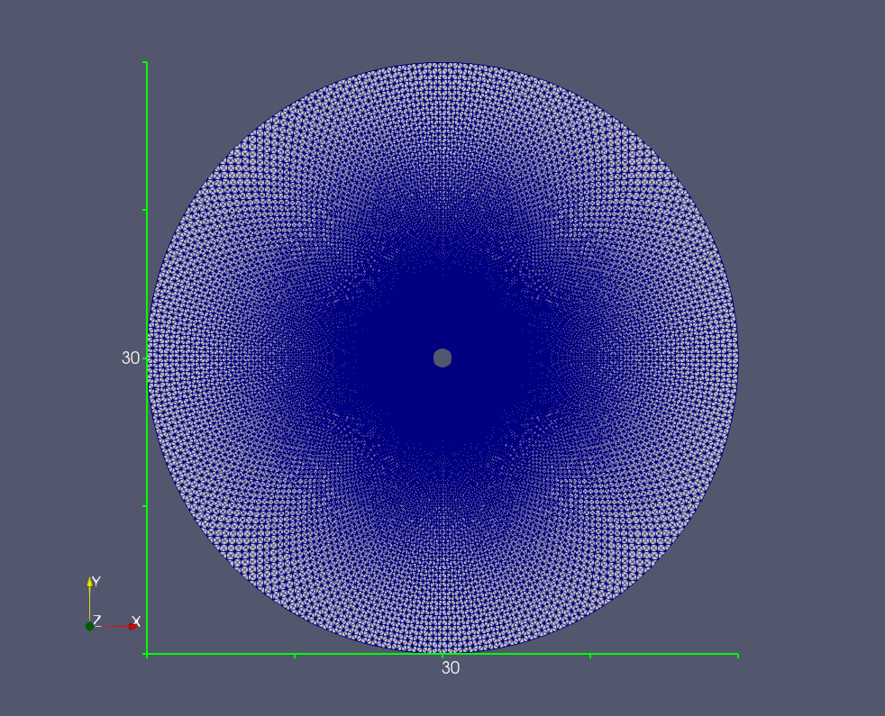
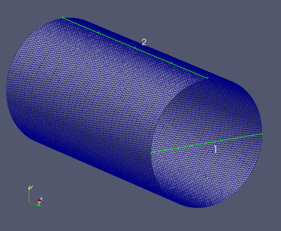
Figure: Cross-sectional view of the global grid (left) and sketch of the mesh on the cylinder wall (right).
2.- Flow around an extruded wing with profile NACA0021
The numerical simulation of the flow around an extruded wing with profile NACA0021 is considered in the proposed benchmark, with an emphasis on the airfoil self-noise generation and propagation. The Reynolds number is set to 0.27 million (based on the chord of the airfoil section) and the angle of attack is 60o. Hybrid turbulence models are good candidates for the simulation of such flows, offering a good compromise between cost and prediction accuracy.
Some views of the computational domain are given in the Figure below. The non-dimensional distance of the first grid nodes is y+=0,7.
The initial flow conditions are ρ0 = 1,225 kg.m-3, Vx0 = V0cos(α) m.s-1, Vy0 = V0sin(α) m.s-1, Vz0 = 0 m.s-1 and p0 = 101300 Pa, where V0 = 34,025 m.s-1 and α denotes the angle of attack (α = 60o).
The inlet turbulence intensity is set to 0.6 %.
The aerodynamic quantities of interest are the bulk coefficients and the pressure distribution on the wing surface, and the root-mean-square pressure fluctuations with regard to the acoustic aspects.
-
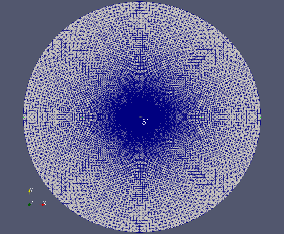
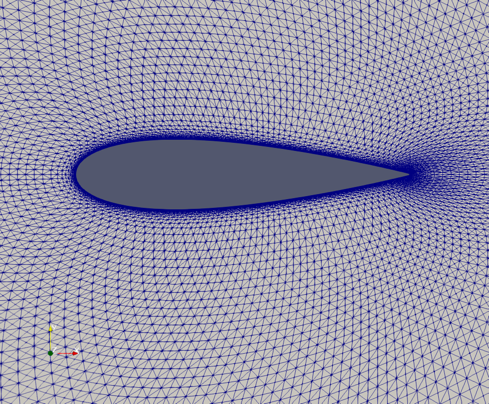
Figure: Cross-sectional view of the global grid (left) and zoom of the mesh around an airfoil section (right).
3.- Rotating cross
The domain is a disk of radius 2 meters and thickness 0.3 meters. A blade of the cross is 1 meter long and 0.2 meter wide. The initial flow conditions are ρ0 = 1, 4 kg.m-3 in the fixed domain, ρ0 = 1,2 kg.m-3 in the rotating domain (see Figure below), v0 = 0 m.s-1 , p0 = 101325 Pa, T0 = 288,15 K and the rotation speed is 1000 rpm.
The flow has to be computed with a turbulence model. In case of a Spalart-Allmaras model, the Spalart variable can be fixed at 10-6 m2 .s-1 at time t=0 s. The physical time for outputs is 0.12 s, this time corresponds exactly to two turns of the cross.
-
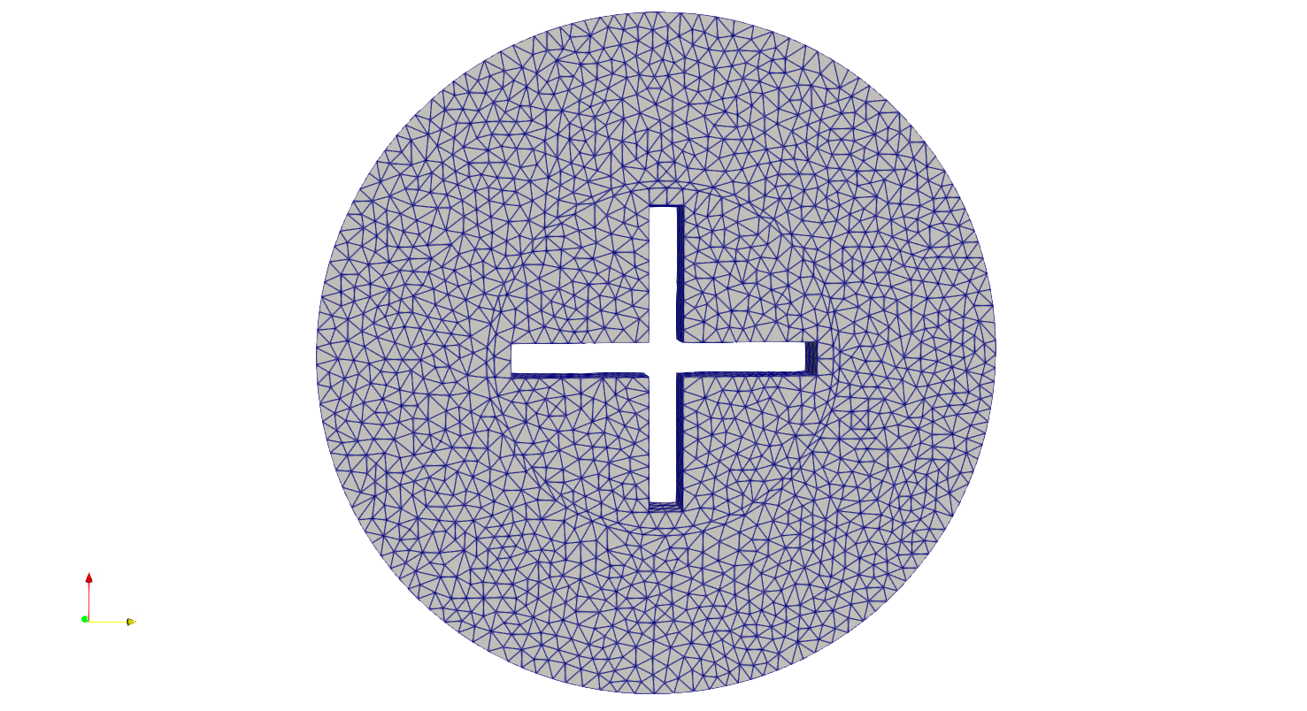
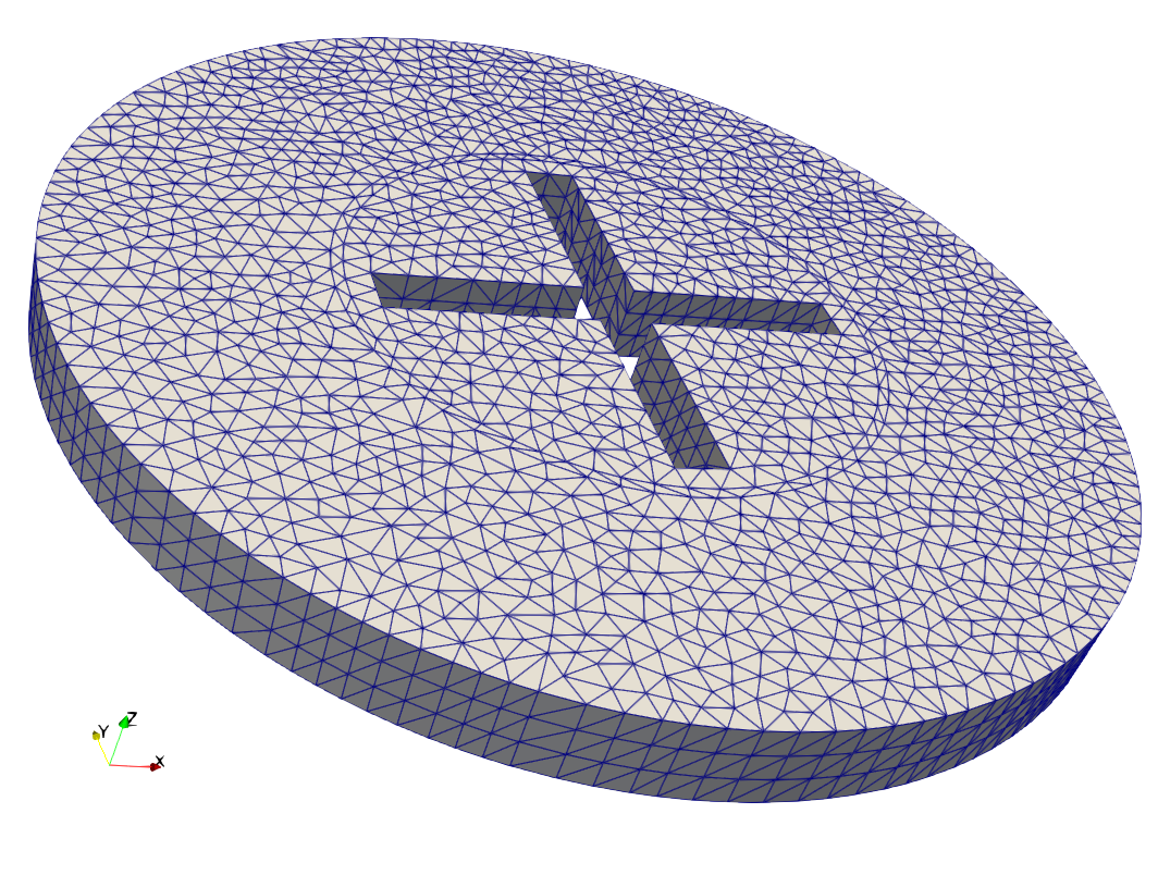
Figure: Sketch of the computational domain with the rotor inside the stator, and a separation to be specified by user, which we have vizualized with two circles.
4.- Flow near a single isolated rotor
This benchmark corresponds to the simulation of the flow around a single isolated rotor and the noise generated by it in the hover mode in a non-inertial rotating frame of reference using hybrid RANS-LES scale-resolving methods. The goal of solving this problem is to compare the scale-resolving methods among partners in application to the simulation of turbulent flow and noise (including broadband noise) in the near and far field. The flow conditions are formulated by Caradonna and Tung [1]. This problem was chosen due to the presence of a large amount of experimental data, including, for a wide range of velocities, the pressure distributions measured in the physical experiment in various sections of the blade, as well as the azimuthal evolution of the position of the tip vortex core. The configuration of the modeled propeller includes two rectangular blades built on the basis of the NACA-0012 airfoil without twist (see Figure below). The blade angle is fixed at 8o. The rotor radius is 1.143 m, the blade chord is 0.1905 m. For the simulation, the axial flow mode was selected at a rotor speed of 650 rpm, which corresponds to a blade tip velocity of 77.8 m.s-1 and a tip Mach number M= 0.228.
-
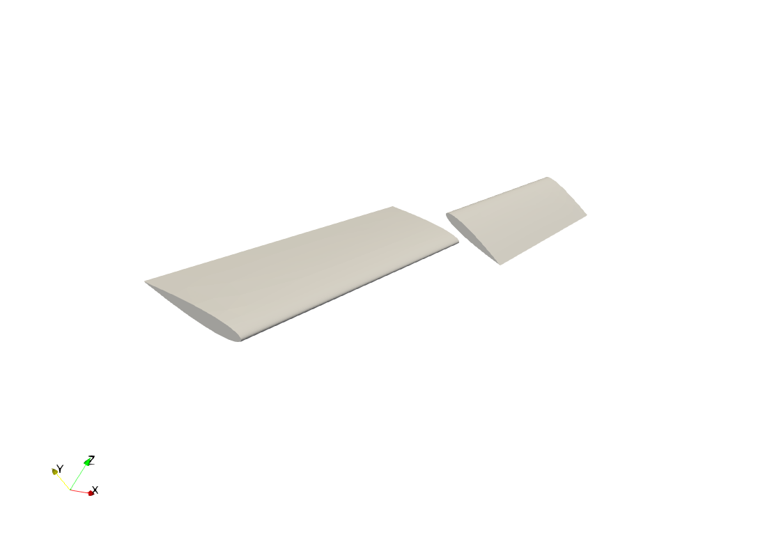
Figure: View of the rotor.
[1] F. X. Caradonna and C. Tung. Experimental and analytical studies of a model helicopter rotor in hover. Technical Report NASA-TM-81232, NASA, Ames Research Center, Moffett Field, California, September 1981.
5.- Rotor+fuselage system
The system of fuselage in presence of rotor can be modeled by combining the rotating Caradonna-Tung rotor with the ROBIN fuselage. See Norma deliverable 'T5-D1: Specification of test cases and first reference calculations (1): single rotor, (2): multirotor' for details.
-
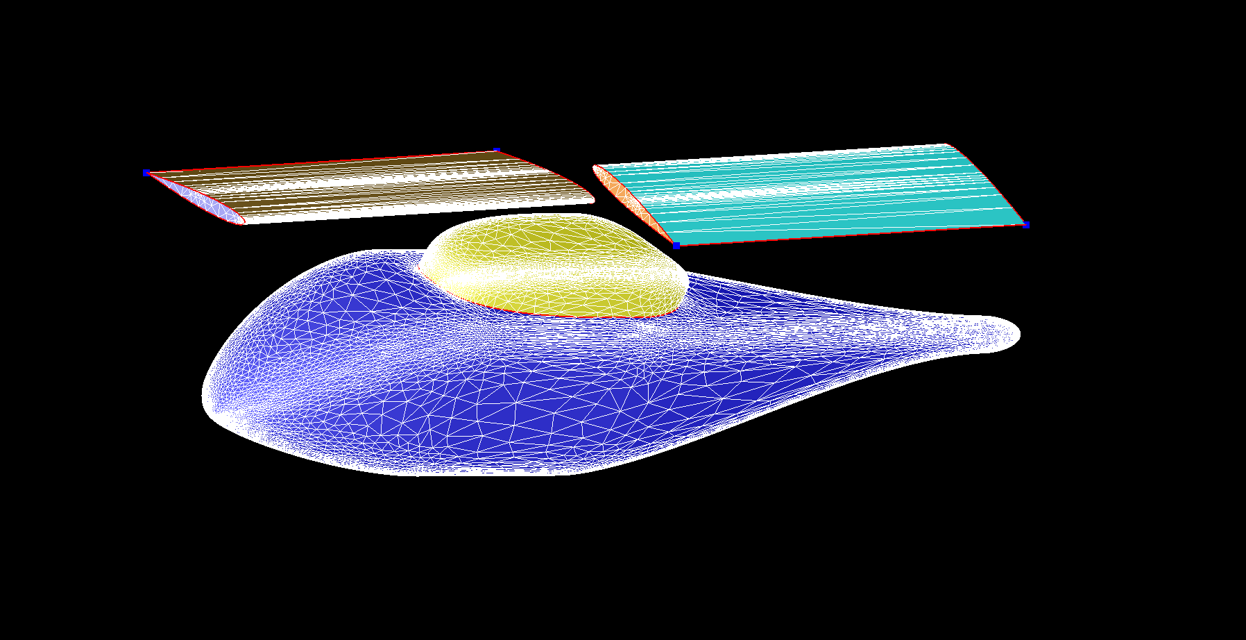
Figure: View of the rotor-fuselage combination.
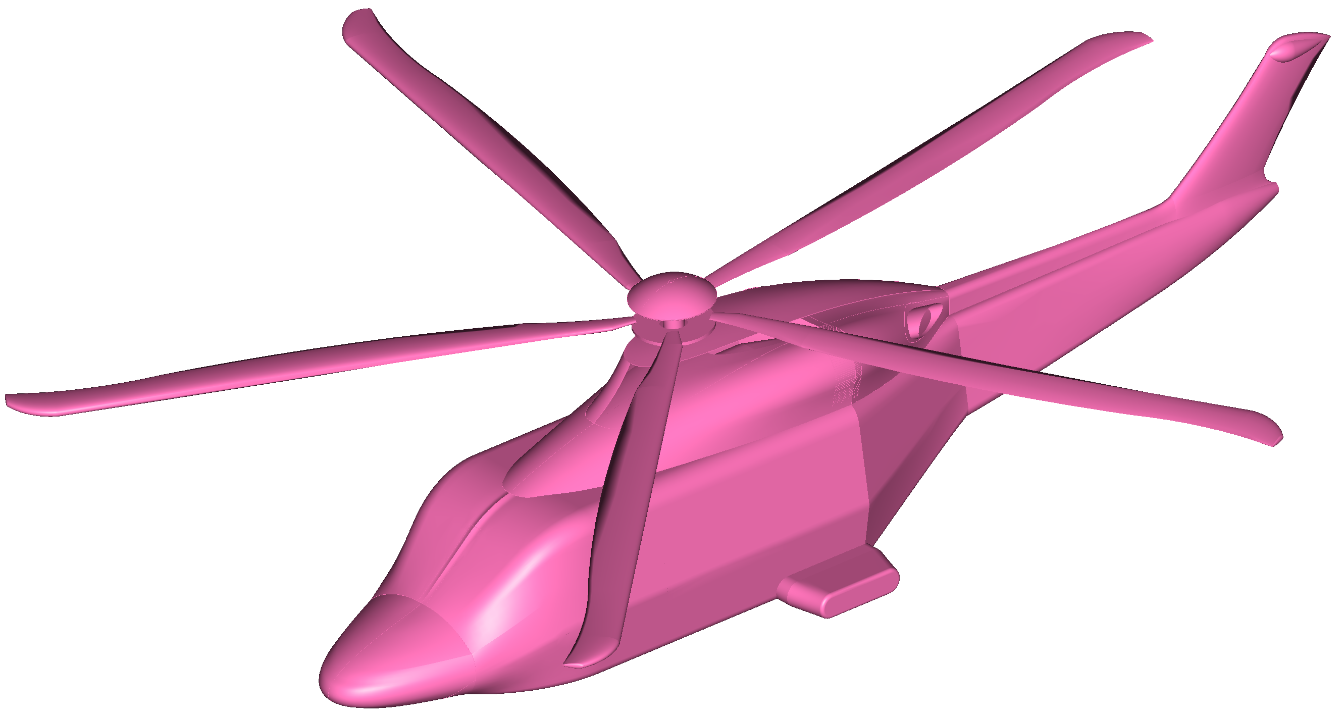
6.- A single-rotor configuration: helicopter with main rotor
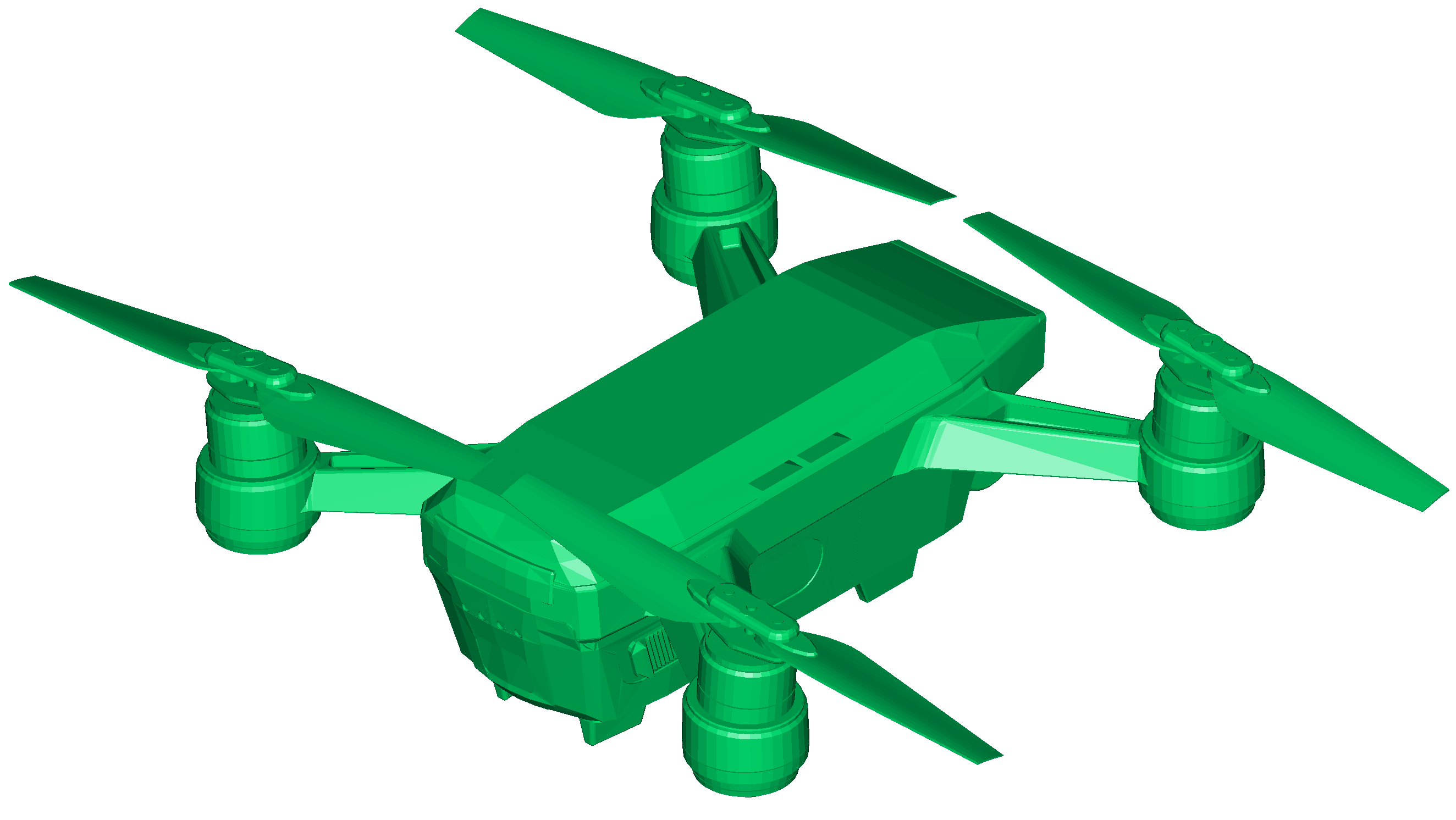
7.- A multi-rotor configuration: quad-rotor unmanned aerial vehicle
Updated mars 4, 2022.